Chapter 8: Distribution, Expectation, and Variance

Suppose we repeatedly observe the same phenomenon:

daily temperature
customer arrivals
stock returns
heights of randomly selected individuals

Each time we collect data, the values are different.

If the data is always changing, what exactly are we trying to learn?

In this chapter we will addressess a fundamental question:

When observed vaules vary from sample to sample, waht remains stable underneath?

Why does Data vary at ALL?¶

let beging with a simple example

import numpy as np

np.random.seed(123)
samples = np.random.normal(loc=167, scale=5, size=55)
print(samples)

[161.57184698 171.98672723 168.41489249 159.46852643 164.10699874
 175.25718269 154.86660378 164.85543686 173.32968129 162.66629799
 163.60556924 166.52645516 174.45694813 163.80549002 164.7800902
 164.82824362 178.02965041 177.93393044 172.02026949 168.930932
 170.68684288 174.45366014 162.32083066 172.87914522 160.73059666
 163.81124249 171.53552598 159.8565965  166.2996564  162.69122552
 165.72190315 153.00705447 158.14233448 163.50061383 171.63731216
 166.13182159 167.01422958 170.44111356 162.60231828 168.41813662
 162.97316741 158.36165253 165.04550103 169.86902931 168.69294525
 166.94084753 178.96182633 169.0645608  171.89368003 178.19071669
 160.52957338 161.80605895 175.71856113 163.00968632 167.14841615]

Even thought all values come from the “same source”, they are not identical.

This leads to an important relization:

Real-word data is not a fixed value repeated many times. It is the output of a variables process.

So the central question of statistics is not:

“What is the value?”

but rather:

“What kind of process could generate values like these?”

What stays table underneath changing Observations?¶

Imagine a hidden machine, each time we press a button, it produces one value. The outputs vary, but not arbitrarily:

some values appear frequently
some are rare
some ranges are likely
others almost never occur

This hidden rule is called a Distribution.

We can simulate different distributions:

import numpy as np
import matplotlib.pyplot as plt

x1 = np.random.normal(loc=12, scale=1, size=1000)
x2 = np.random.normal(loc=15, scale=3, size=1000)


plt.hist(x1, bins=30, alpha=0.6, density=True, label="std = 1")

plt.hist(x2, bins=30, alpha=0.6, density=True, label="std = 1")

plt.legend()
plt.title("Different distributions generate a different data pattern")

plt.show()

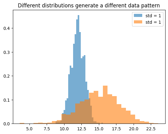
The dataset is what we observe, the distribution is what generates it.

If a Distribution is a Rule, How do we Summarize it?¶

Suppose we collect thousands of observations.

What are the first things we want to know?

Typically:

1. Where do the values tend to center?
1. How much do they vary?

Statistics formalizes these two ideas as:

Expectation(mean)
Variance

Where does the Data tend to Center?¶

If we repeatedly sample from the same process, the average value stabilize.

This long run average is called the expectation.

x = np.random.normal(loc=78,scale=4.5, size=10000)
print(np.mean(x))

78.09808626147

This approximates:

E[X]

(1)

Important distinction:

$E[X]$ : property of the distribution(unknow)
Sample mean: computed from observed data.

The expectation belongs to the underlying process.

The sample mean belongs to the data we observe.

Why is the mean Not Enough?¶

Consider two datasets:

x1 = np.random.normal(0, 1, 1000)

x2 = np.random.normal(0, 5, 1000)

print(np.mean(x1), np.mean(x2))
print(np.var(x1), np.var(x2))

0.046977642284805 0.10531909321746996
1.1003530403293311 23.700346021488112

Both have similar means, but very different spreads.

This shows:

Knowing the center alone is not sufficient to describe a distribution.

We also need to measure variability.

This leads to variance.

Variance measure how much values deviate from expectation.

Interpretation:

Small variance -> values are tightly clustered
Large variance -> values are widely spread.

Why do large samples looks more stable?¶

Individual observations fluctuate, yet averages become more stable as we collect more data.

Why

Let simulate this

means = []

for n in range(1,500):
    x = np.random.normal(165,3,size=n)
    means.append(np.mean(x))

plt.plot(means)
plt.axhline(165)
plt.title("Sample mean stabilizes as sample size increase")
plt.show()

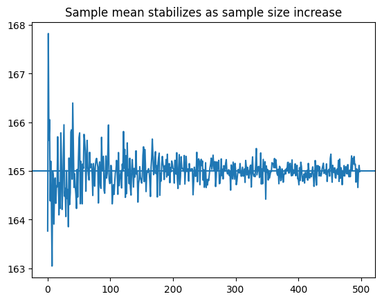
Observation:

Small samples -> high variablility
Large samples -> stable averages

This phenomenon is know as the Law of Large Numbers.

Are all Distributios the same?¶

Not all variables behave in the same way.Some variables take discrete values:

coin flips
number of arrivals

coin = np.random.binomial(1,0.5, size=40)
print(coin)

[1 1 0 0 1 0 0 1 1 1 1 0 1 0 0 0 0 1 0 1 0 1 0 1 1 0 1 1 1 0 0 1 0 0 0 0 0
 0 0 1]

Others take continuous values:

height
temperature

height = np.random.normal(170,8,size=40)
print(height)

[169.41720832 162.03902962 165.86728701 172.28724762 182.91277197
 167.1105468  173.90954729 163.75158168 156.28566275 182.49395581
 164.05667483 162.89527223 156.25050178 155.4517775  172.34642592
 174.10743123 164.9324674  161.6601461  188.83761201 181.14312659
 173.12464219 159.22947084 156.82138983 161.915582   176.60344802
 182.17082555 177.73620024 160.2667046  147.93050686 177.22225635
 162.15258497 173.5098158  176.77100032 175.19913064 169.37330901
 163.64875439 177.49287683 179.48005318 169.00368423 183.79347153]

Cenceptually:

Discrete distributions assign probability to specific values.
Continuous distributions assign probability to range.

Why does machine learning care about distributions?¶

Machine learning is often described as "Learning patterns from data"

A more precise statement is:

Machine learning attempts to approximate the underlying distributino.

Examples:

Regression aims to estimate:
$E [Y |X]$
(2)
Classification aims to estimate:
$P(Y|X)$
(3)

These are not arbitrary constructs.

They are properties of the data-generating process - a model is a simplified representation of the true distribution.

What are we really learning?¶

We return to the original question:

If observed values keep changing, what are we actually trying to learn?

we are not trying to memorize individual observations, we are trying to understand the structure that generates them.

A distribution describes how data is generated
The expectation describes its center

Statistics begins when we move from individual observations to the hidden structure that produces them.