Chapter 9 Covariance & Correlation

In the pervious chapter we asked:

• When data varies, what remains stable?

We answered:

• A distribution describes how values are generated

• The expectations gives the center

• The variance gives the spread

However, we made one critical simplification:

• We only looked at one variable at a time

The New Problem¶

Real data is almost never one-dimensional

instead, we observe multiple variables simultaneously:

• weight and height

• temperature and electricity demand

• study time and exam score

• price and demand

This raises a new question

If each variable has its own distribution, how do variables behave together?

The core question of this chapter¶

When mulitple variables vary, what structure governs their relationship?

observing joint variation¶

First let’s start a simple example.

import numpy as np 
import matplotlib.pyplot as plt

x = np.random.normal(0,1,1000)
y = 2 * x + np.random.normal(0,1,1000)

plt.scatter(x,y, alpha=0.3)
plt.title("Two variables varying together")
plt.xlabel("X")
plt.ylabel("Y")
plt.show()

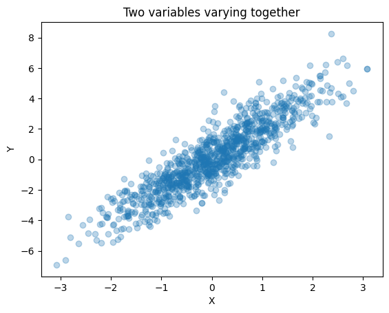
We observe:

• x varies

• y varies

• but they are NOT INDEPENDENT There is a pattern.

Why mean and variance are NOT ENOUGHT¶

From Chapter8:

• mean tells us where values center

• variance tells us how much they spread

But now we have two variables,questions we can not answer using only mean and variance:

• When x increase, does y increase?

• Do they move together or independently?

• How strong is their relationship?

This leads to a new concept:

We need a way to measure joint variation.

Introducing Covariance¶

We define:

• Covariance measures how two variables vary together

Intuition:

• If x and y increase together -> positive covariance

• If one increases while the other decreases -> negative covariance

• If they move independently -> covariance near zero

print(np.cov(x,y))

[[1.0645908  2.12158412]
 [2.12158412 5.21164557]]

Conceptually:

• Covariance measures whether deviations from the mean occur together.

If x is above its means and y is also above its mean -> positive contribution

If one is above and the other below -> negative contribution.

Key interpretation:

• Positive convariance -> variables move together

• Negative convariance -> variables move oppositely

• Near zero -> no linear relationship

Why convariance alone is NOT ENOUGHT¶

Covariance depends on scale.

For example:

• measuring height in cm vs meter changes covaiance

• measuring income in dollars vs thousands changes covariance

This mankes raw covariance difficult to compare.

Correlation: A standardized measure¶

To address this, we normalize covariance.

• Correlation is a scale-free measure of relationship

Properties:

• range between -1 and 1

• unit free

• directly interpretable

np.corrcoef(x,y)

Interpretation:

• +1 means perfect positive relationship

• 0 means no linear relationship

• -1 means perfect negative relationship

Visual Interpretation of correlation¶

We can compare different relationships

x = np.random.normal(0,3,1000)

y1 = x + np.random.normal(0,0.5,1000)
y2 =  np.random.normal(0,3,1000)
y3 = -x + np.random.normal(0,0.2,1000)

fig, axs = plt.subplots(1,3,figsize=(12,4))
axs[0].scatter(x,y1,alpha=0.3)
axs[0].set_title("Positive")
axs[1].scatter(x,y2,alpha=0.3)
axs[1].set_title("No relationshipe")
axs[2].scatter(x,y3,alpha=0.3)
axs[2].set_title("Negative")
plt.show()

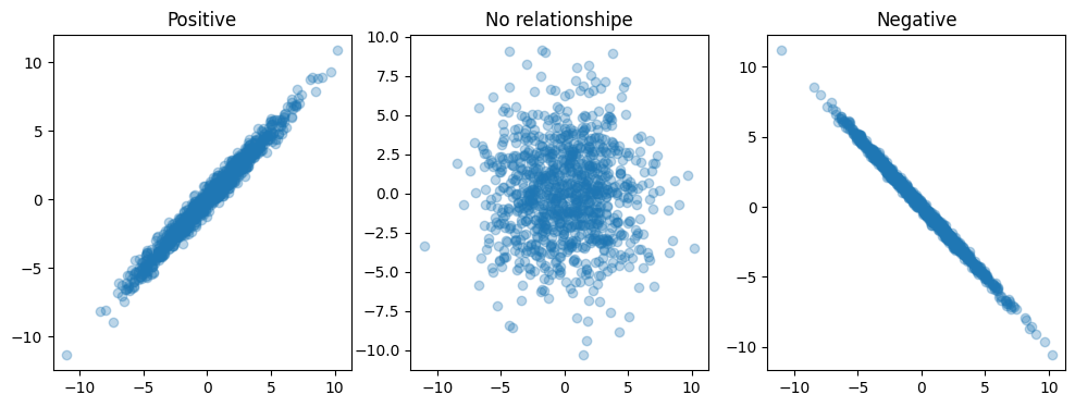
Observation:

• correlation captures the direction and strength of linear relationship

From pairwise relationships to structure¶

So far, we have considered two variables,in real datasets, we often have many variables.

We can compute a covariance matrix

data = np.random.multivariate_normal(
    mean=[0, 0, 0],
    cov=[[1, 0.8, 0.5],
         [0.8, 1, 0.3],
         [0.5, 0.3, 1]],
    size=1000
)

np.cov(data.T)

This Matrix summarizes:

• variance of each variable(diagonal)

• covariance between variables(off diagonal)

Why this matters in Machine Learning¶

Many machine learning methods rely on relationshipe between variables. Example:

• Linear regression: models how variables influence each other

• PCA: finds directions of maximum covariance

• Feature selection: removes redundant(heighly correlated) variables

This leads to broader insight:

Machine learning is not only about individual variables, 
but abount the structure formed by their relationships.

Summary¶

We return to the central question:

• When multiple variables vary, what structure governs their relationship?

The answers is:

• covariance describes how variable vary together

• correlation provides a standardized measure of that relationship

• the covariance matrix captures the overall structure

Statistics is not only about variation, but about structured variation.